Formula Electric (FSAE)

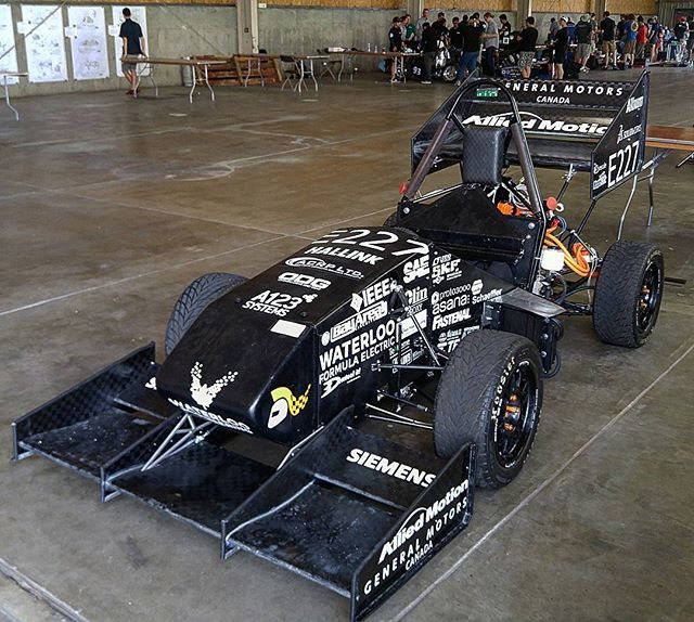
When I returned to school after running Embark, I joined the Formula Electric team and quickly became engineering and product lead for the new season. With too few subteam leads, I also led the control-algorithms and accumulator (battery pack) teams while leading the 2018 car’s architecture and design. That meant building simulation tools so every area could make data-driven decisions.

After eight months I stepped back to focus on other priorities, and kept consulting for the team where needed.

Running a startup had taught me a lot about building an effective organization, and I pushed to change how the team worked. I built a Confluence wiki and a culture of continuous documentation so knowledge carried over year to year, and set up project outlines and deadlines there so leads could hand well-defined projects to students each term.

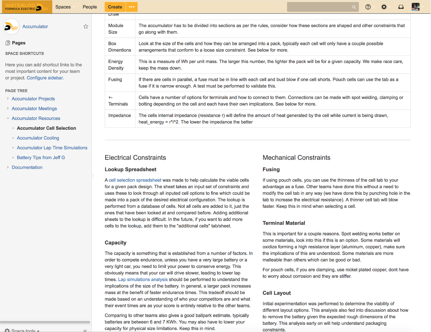
I also worked on how the team ran meetings, mentored newer members and resolved conflict. Over the season the team grew from 20 to 50 members, and annual sponsorship tripled.

Choosing the 2018 architecture meant understanding trade-offs like power-to-weight, battery capacity against mass, and aero cost against performance. Existing simulators were too simplified and couldn’t evaluate torque vectoring with independent motors per wheel. Most ignored weight transfer, which decides when each tire loses traction.

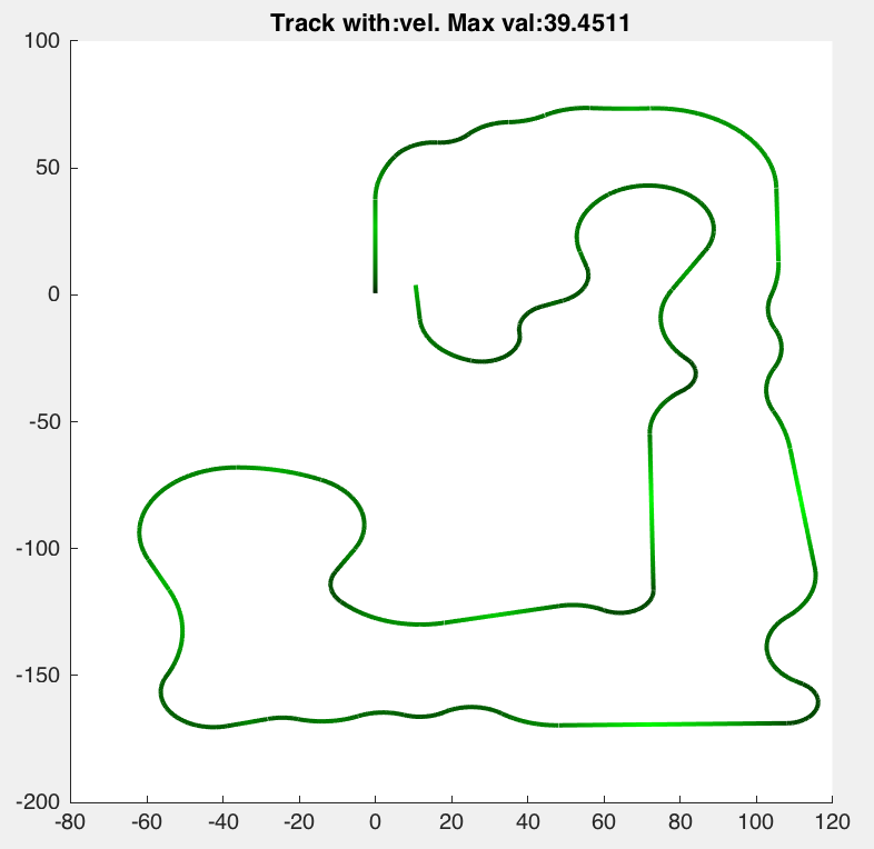
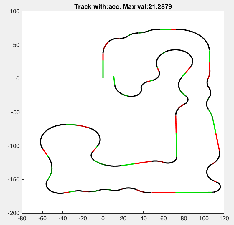
So I wrote one in Matlab: a point mass limited by a friction ellipse, driven through a track of arcs and straights, accelerating and braking at the theoretical limits while aero drag and downforce change with speed. At about two seconds per lap, we could sweep parameters in batches and build trade-off maps to decide where to spend effort.

The plots below show one simulated lap, coloured by velocity and by acceleration.

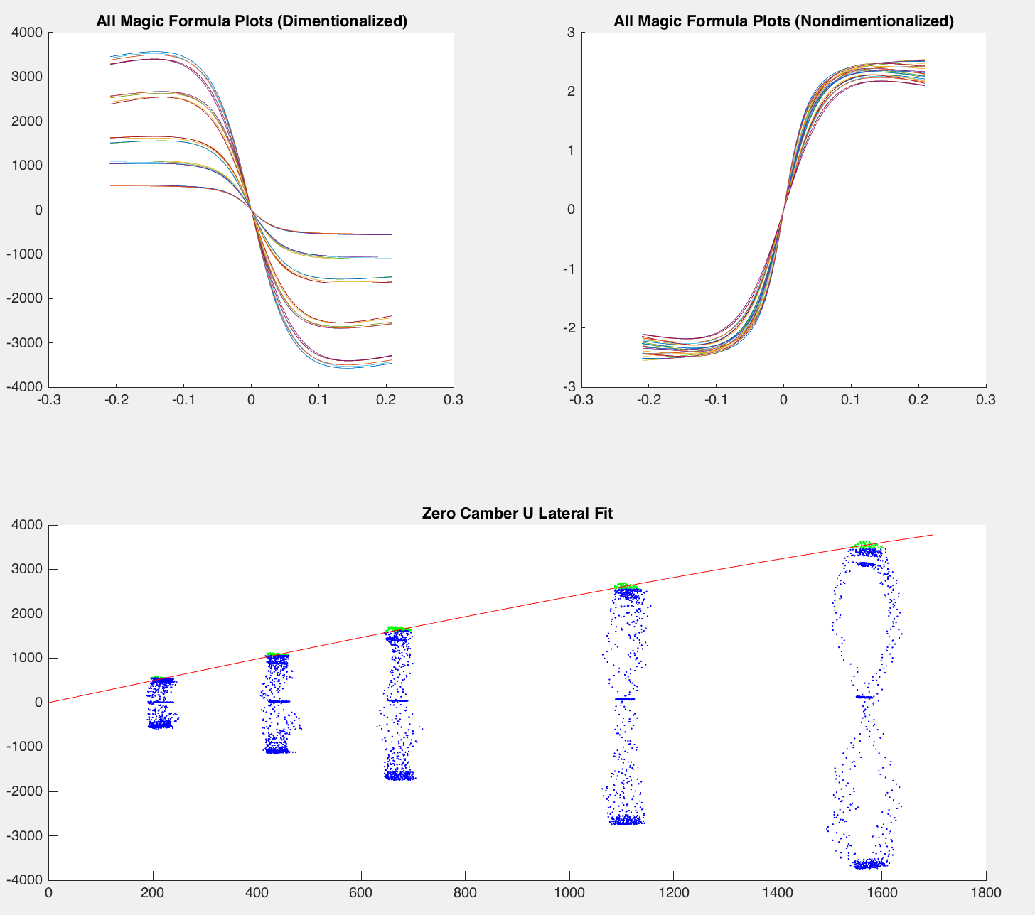
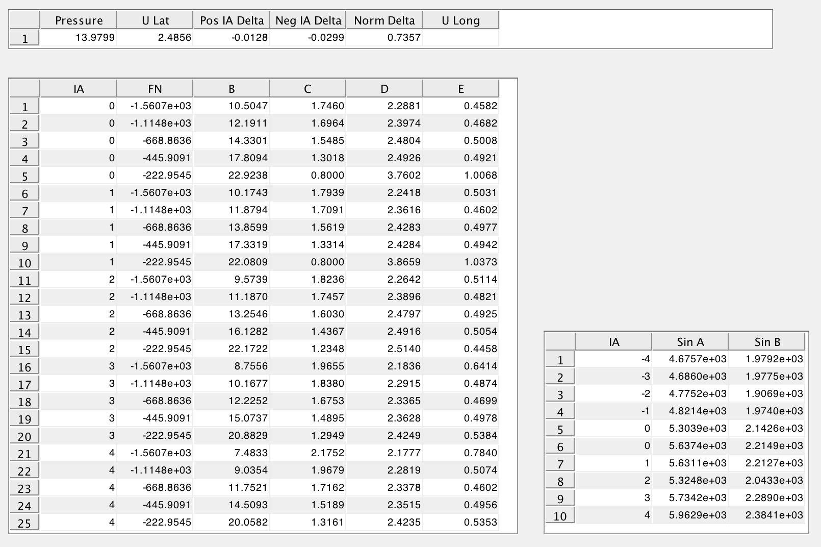
Tires set the limit on every force a car can use. Paying a firm to test tires would have cost too much, and testing them ourselves would have taken too many people, so we used the raw test data a group of former FSAE members publishes each year. Turning it into usable coefficients usually means a $1,000 tool. I wrote a Matlab script instead that splits the logs into individual tests and fits:

1. A standard tire model to slip angle versus lateral force, for varying camber and normal load.
2. Lateral and longitudinal friction coefficients as functions of the test parameters.
3. Other data, like returning force, formatted so it’s easy to extract.

The script presents the results as plots and tables. In the fits, the top two plots overlay every fitted curve, dimensional and non-dimensional, and the bottom one fits the lateral friction coefficient at zero camber.